
Differential Equation Labs
After four semesters teaching different applications of Differential Equations concepts at Purdue's Recitation section through computational laboratories, I want to share some hints and advice to aid your understanding of the concepts and interactions with the software in each lab. You could also find additional information about the labs as well as the problems in the Project Rhea Website.
In terms of grading, just make sure to check the rubrics as shown in the Rhea website's lab table to have all the required information in your submitted file to be graded. Also ensure that all your problems and graphs are labeled. I recommend having your labs in a typeset document (Word or Google Docs) with all the necessary details (screenshots, pictures, and equations) for each problem to convert as a PDF.
Lab 0 – Introduction
Logistics
All the software can be downloaded unto your personal computers, although they are also available on the classroom desktops. Dfield and Pplane can be downloaded on this site. There is also an online alternative that incorporates both Dfield and Pplane (one and system of two ODEs) features by Bluffton University. Matlab and Maple can be accessed remotely through the go remote site with your Purdue Credentials, or can be downloaded through Matlab and Maple.
DO NOT FORGET to please fill out the Lab 0 form. Although the lab is not to be submitted, the form is. Read the syllabus at your own time and get familiar with the different platforms the class will be utilizing, i.e., Brightspace, the Project Rhea Page, and the different softwares (DField, PPlane, Matlab, and Maple).
Advice
The main goal of this lab is to help you get familiar with the tools we will be working on throughout the semester. Do not worry if you do not feel comfortable during your first go at the different softwares as we will emphasize the important details next lab. The main takeaways are:
- how to plot in DField, PPlane, and Matlab (with fplot)
- the Keyboard Input to plot a specific solution onto PPlane and DField
- zooming in and out on these sofwares
- the inference process to find the different solutions.
The underlying code to follow along in Problem 5 is as follows:
>>  grid on
    hold on
    xlim([–10,10])
    ylim([–10,10])
    fplot('x*exp(–2*x)+x^3+cos(pi * x) + 1', 'g');
Lab 1 – CSI for an Hour
Overview
The analysis of thermodynamical systems using differential equations is a fundamental approach in physics and engineering. Think of thermal equilibrium in the same way radiative decay was studied in high school, the more time elapses, the slower an object cools down. This occurs because the closer in tempreature two bodies are, the slower they exchange heat to reach equilibrium. In other words, the rate of temperature of two bodies varies on their temperature difference. The smaller this difference is, the slower the temperature change rate is.
For our analysis, let us set the bodies to be a room and an object in a room, where the temperature we are interested is of the latter, denoted as T. Fix the object's temperature to be colder than the room's temperature R. From our past discussion, becuase the rate of change is proportional to the difference, let k represent the constant that relates the difference to the rate (we wish for it to be positive). Thus, we can express this behaviour as,
Problem Statemet
How can we relate the discussion above to a corpse laying in a room with no clear idea of how long it was last alive? Well, we can let the object in our analysis to be the corpse while we replace R with the value of our circumstance. Firstly, we need to approximate the value of k, which can be easily done with two measurements, then we can relate the equation to our initial input values from our mesaurements. For the picture to become clearer, try it yourself doing the problems in the lab which go into more detail.
Main Takewaways
- Ensure that the variable naming is consistent with the notation we have in our labs to avoid confusion. Having the proper independent and dependent variables while ensuring the parameter names are different from the variables.
- There are multiple ways to enter constant parameter values in Dfield. Throughout the semester, I will enter the parameter values in the Parameter Expressions section where it is easier to alter constant values.
- Remember to alter the display window range according to the analysis. In this case, our analysis ranges for
Tat most 100° but no lower than 70°, meanwhiletis between -5 and 5 as time is offset ±5 hours from midnight.
Common Confusion
Problem 8 is usually confusing at first, think about it in terms of the following timeline.
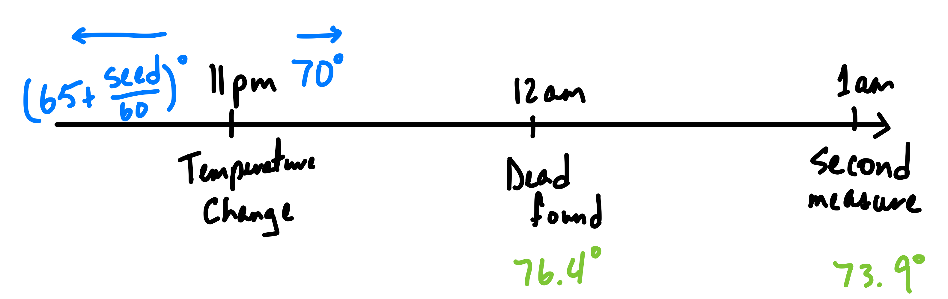
So far, we have been treating midnight to be
where we made our first measurement of the temperature. However, now at time
11pm, there is a discontinuity in the temperature of the room. So we need to relate
and
in terms of their respective initial values for our problem.
First, we need to backtrace the temperature of the body at the moment of the temperature change. This value would become the T initial value of . It is simpler to keep
t as the value from our initial continuity, i.e., -1. From this new resulting curve, we can approximate when the body was last alive with a 98.6°F body temperature, as done in previous problems. Remember to add from midnight this t value to see the approximate hour of the day the body was last alive.
Lab 2 – Understanding Escape Velocity
Logistics
This is the first lab that has presentation assignments. I will use this as a reminder that presentation notes are due Monday night before your presentation assignment. For example, if you are assigned Problem 5a from lab 2, and we are discussing this lab next Tuesday, email and submit through Brightspace your notes by next Monday so I can comment and correct if necessary. Refer to Brightspace if you are wondering what problem you have been assigned for your presentation. All the dates corresponding to them are described in the same table as well.
Overview
Gravitational problems are a common place to understand differential equations relating position, velocity, and acceleration together through simple derivatives. This simple, yet insightful, type of problem can show how systems of equations builds a bigger picture that could be easily overlooked when expressing equations in one. Problems 1 and 2 show this principle visually through Dfield and Pplane. Dfield is limited to one differential equation, while Pplane can work with systems of differential equations with two dependent variables.
Advice
For Problem 3, please build a table with the underlying information. The template would be something like
| v(0) | Height (y) | Height (x, i.e., miles) | Velocity (v) | Velocity (mi/s) |
|---|---|---|---|---|
| 0.5 | (value/N) | (value/N) | (value/N) | (value/N) |
| 1.0 | (value/N) | (value/N) | (value/N) | (value/N) |
| 1.5 | (value/N) | (value/N) | (value/N) | (value/N) |
| 2.0 | (value/N) | (value/N) | (value/N) | (value/N) |
where (value/N) stands in for either N when it does not apply or value for the approximate value from the graph in the appropriate units. The does not apply stands for when there is no maximum height (it leaves Earth) or if there is no velocity at escape (it fell back to Earth).
For Problem 5, recall basic Algebra, Calculus, and the course for evauluation through substitution, limits, and first order differential equation solution of seperable variables.
Problems 6 and 7 are the most time consuming problem in the lab. Trying to patch our understanding of escape velocity with air resitance as an additional force in the system. Algebraically, the air resistance only affects the second order derivative through Newton's Second Law of Motion. Based on this, we can find the position equation in terms of y through integration and initial values to find the constant of integration. Their template MATLAB code (replacing their appropriate fplot equation) is:
>>  grid on
    hold on
    fplot('100*x-10^4*log(1+0.01*x)-1')
Common Confusion
Our variables for position are x and y while time is in terms of t and s. Treat x and t as your real units (mile and second respectively) variables while y and s are imaginary unit variables used to simplify calculations. Thus, we have to constantly convert our results to tangible units (x and t). The basic conversions are given by
The confusion arises when differentiating, which by chain rule differentiation we have,
Recall that v is our independent variable which is given by
and that
and
are constants calculated from the equations above. Therefore, to build the table in Problem 3, we only need the equation for
, the evaluation of constants, and
v value.
Lab 3 – Existence and Uniqueness Theorems
Introduction
It is incredibly crucial to understand the two theorems foundational for our discussion:
Existence Theorem
If
is defined and continuous on a rectangle
in the tx-plane, then given any point
the initial value problem
has a solution
defined in an interval containing
Uniqueness Theorem
If
and
are both continuous on a rectangle
in the tx-plane,
and if both
and
satisfy the same initial problem
and
then as long as
and
stay in
, we have
Useful Test
One powerful test to wrap our minds around such a abstract concept is as follows:
Let
and
then ask,
- Can we choose an open rectangle that contains
such that
is continuous?
- Can we choose an open rectangle that contains
is continuous?
If question one is true, then Existence Theorem applies. If both are true, then Uniqueness Theorem applies.
Analytical Examples
Existence does not hold
-
and any
.
-
Similarly,
and any
Although, this case is much more interesting because plotwise, it seems like there exists a solution by choosing either of two functions such that its corresponding unilateral limit is zero, i.e,
Uniqueness does not hold
-
-
and any
.
Biggest Takeaways
Converse – Problem 2
Note that their is an intentional word choice to describe the theorems and whether or not it holds. This is because the converse of each theorem is not necessarily true (I am not sure if the converse of Uniqueness is, as I could not find or think of a counterexample but Existence Theorem's converse does not hold). An easy example is covered in Problem 2 with
where Existence Theorem does not hold (and by consequence Uniqueness does not either) for any t=0.
When solving through the Separable Method, we find
for the constant of integration based on the initial value. Therefore, if we define the initial value to be given by
we can see that there exists infinitely many C values that satisfy the system.
Uniqueness Neighborhood – Problems 3 & 4
It is quite easy to overlook the fact that the Existence Theorem does not give insight to how the existing function might behave like. In other words, the only properties we know of the solution functions are given by the initial conditions we start off with, and we will not be able to get any additional properties outside of the neighborhood (rectangle R) without considering other initial values. Which is why Problem 3 might seem counterintuitive at first as we are told a solution exists but when we evaluate the function at a different point
then
might not exist. Furthermore, evaluation of the function at any point outside of the initial value's neighborhood is indifferent from the previous analysis. For example, as done in Problem 4, we could define the parts of the solution function somewhat arbitrarily (like our age) if we are careful with the section changed to avoid violating any of the theorems by keeping x'=f(t,x) intact. For a helpful formulation BYJU's explanation on the Uniqueness Theorem is quite helpful. The most important fact is that the Uniqueness Theorem ensures the uniqueness of the solution if the interval (rectangle) is not so large.
Geometric Implications – Problem 5
After showing that the functions are solutions to the differential equation, let us analize what we know. The function f(t,x) that follows,
holds Existence and Uniqueness Theorems at all points except
Notice, the problem is referring to the unaltered satisfying function called x(t), in any rectangle of its domain. Thus, given that it is trivially shown the constant functions y(t)=0,2,4 regardless of t are solutions, by Uniqueness Theorem, we can argue that x(t) cannot cross or intercept y(t)=0,2 as the initial value is in that interval. Therefore, we can conclude the bounds are 0 and 2.
Lab 4 – Linear First Order Differential Equations
Introduction
This lab is very unusual to all others throughout the semester. We will be utilizing Maple, which is an incredibly powerful tool to process algebraic analysis without the need of manual arithmetic manipulation. Maple Help is an incredible resource for the standard functions and syntax of the language. Its applications are incredibly diverse, and the website contains an in depth description of applications in a variety of fields, including a manual section for Differential Equations. The main things to understand of this lab is the syntax and main functions is also shown in the discussion section of the handout which I can summarize, as below.
Main Syntax and Functions
- To generate a variable, we can just name it as you wish, and utilize the
:=to denote it from its evaluation. For example,
example := (expression)
-
To denote a differential, i.e,
the function
diff(f(t),t)is employed. While integration is done with theint(f(t),t)function, which disregards the integration constant. -
With these two main points we can then build differential function variables, like
equation := diff(exp(2*x),x) + x^2*y
where
exp(x)
represents the exponential
function.
- To solve a differential equation by an initial condition, we utilize
dsolve({equation, y(x_0)=y_0}, y(x))
# x_0 and y_0 are the given initial conditions
Other useful solving functions:
- Left and right hand side
lhs()rhs(), respectively, to help extract information from an expression. simplifywhich applies simplification rules to an expression.subs()is used to substitute expressions for others.
Note, we have to specify the structure of the function by its dependent and independent variables in all of the functions. To ensure all command lines are executed properly, I would recommend entering them one at a time. For example, if the complete code segment is pasted, and hit enter once, I have encountered it would not simplify expressions correctly. For evaluation puposes, it is also best to ensure every line is printing the expected result.
Code
Problem 1
First, let us define our differential equations to work with as shown in the handout. To find the solutions given their initial input, we then utilize dsolve(). This should print the resulting function.
#1
equ1 := (x^2 + 1)*diff(y(x), x) + 3*x*y(x) = 6*x;

dsolve({equ1, y(0) = -1}, y(x));

equ2 := diff(y(t), t) = (-2*t*(1 + y(t)^2))*1/y(t);

dsolve({equ2, y(0) = 1}, y(t));
Problem 2
For the first part of the problem, we will need to define the (**) differential equation. Then, we can build functions that solve the differential equation for different initial values, which we will call f and g. For this, we would need to find the initial value solution with dsolve(), and extract the solution with rhs() to define our functions with the proper := syntax.
#2a
equ := diff(y(x), x) + x^3*y(x) = x^3;

f(x) := rhs(dsolve({equ, y(0) = 2}, y(x)));

g(x) := rhs(dsolve({equ, y(0) = seed}, y(x)));
To print the results, just type the name of the function, for example,
f(x)
and it outputs the explicit value of the solution to the system. Please make sure f and g are printed for your submission.
For 2b we are interested in substituting our functions back into the equation to verify they are solutions. Given the variable equ has two sides, we can substitute it on the left hand side expression, then simplify to verify both sides of the equality hold.
#2b
subs(y(x) = f(x), lhs(equ));

simplify(%)

subs(y(x) = g(x), lhs(equ));

simplify(%)
I would argue the next subproblems are the main takeaway of the lab. Recall linearity of differentiation, meaning the derivative of a sum of functions is equivalent to the sum of their derivatives, nice properties emerge to build a possible subset of solutions to first-order differential equations. One such case is the difference and sum of solution functions to a homogeneous first-order equation.
Let us prove the difference of functions hold a solution, as we can repeat the same process from before to a generically solved defined functions, f and g, to build the difference. Thus, we can run the following:
#2c
h(x) := f(x) - g(x);

subs(y(x)=h(x), lhs(equ))

simplify(%)
Hopefully it is evident why more generally for the same where, if there are two distinct functions whose differential expression simplify to the same function, their difference also solves the homogeneous differential equation of the expression. The previous claim implies the difference of two functions which solve a non-homogeneous first-order differential equation at different initial values would also solve the homogenous differential expression.
To prove this sub-claim, as requested by the problem, we would do similarly as the previous proof, generalize to any non-homogeneous equation with equd and find different initial values, then expresses as follows to find it simplifies to zero as well,
#2d
equd := diff(y(x), x) + p(x)*y(x) = q(x);

f(x) := rhs(dsolve({equd, y(0) = a}, y(x)));

g(x) := rhs(dsolve({equd, y(0) = b}, y(x)));

h(x) := f(x) - g(x);

subs(y(x) = h(x), lhs(equd));

simplify(%)
Another nice property is that the sum of a solution to a first-order homogeneous differential equation and a function that satisfies the non-homegeous expression case, also solves the non-homogeneous first-order differential equation. Let us define as before with g and yc, this should simplify to the value of q(x), in this case,
#2e
g(x) := rhs(dsolve({equ, y(0) = b}, y(x)));

equh := diff(y(x), x) + x^3*y(x) = 0;

yc(x) := dsolve(equh, y(x));

F(x) := yc(x) + g(x)

subs(y(x) = F(x), lhs(equ));

simplify(%)
We can then wrap Problem 2 up by showing they express the same solution set as all solutions are a coefficient of exp(l(x)) away for the smae l(x). We can verify with,
#2f
dsolve(equ, y(x))
Existence and Uniqueness, again
Last week we discussed the Uniqueness and Existence Theorems, and this lab tries to make sure we understand the real implications of these theorems. First we can emphasize how the properties of the solution functions, for example where it ceases to exist (its domain), vary from initial conditions. However, we also generalize the theorems to any first-order differential equation:
If
and
are both continuous on the interval
which contains,
then the initial value problem
has a unique solution
which exists for
and any value of
Note, we can express this equation to satisfy the Uniqueness and Existence criteria discussed before. Hopefully, once converted, it is self-evident the explanation for its behavior. We then can wrap up with an example showing how satisfying the previous theorem is sufficient to show existence and uniqueness, but not necessary, as I also clarified last lab. Just because p and q become unbounded, does not imply that the solution function also is unbounded in the same region.
Lab 5 – Modelling Population
Introduction
After some theory discussion, Lab 5 will start with the first lab within our mathematical modeling saga. We will learn to use some mathematical models that can help us build predictions based on data. We will learn about the following three different prediction models for population growth:
- Linear
- Exponential
- and Logistic
We will also try to objectively determine which model is the best representation of the data. The most important detail to know of the models, is that t is going to represent in our function P(t) the number of decades after 1790, making our initial sdata point t=0 to be that same year.
Code
Problem 1
First, we will import the data into Matlab for better plotting and analysis. The first line is shortline to build an array from 0 to 20 by adding one to each element. Then, we define explicitly the data, such that its corresponding index is t (i.e., P(t=0)=379). Afterwards, we can plot these points on a grid with the plot function to build a piecewise red 'curve' specified by the third argument.
>>T = 0 : 1 : 20;
>>A=[379, 423,472, 523, 610, 738, 995, 1231, 1457, 1783, 2239, 2805, 3366, 3852, 4250, 4317, 4691, 5149, 5689, 5737, 6016];
>> grid on
>> hold on
>> plot(T,A,'r')
Problem 5
After solving for the different population functions based on the models, we can plot all these equations (in the code the first argument is the function while the second specifies the color).
>> fplot('44*T+379','g');
>> fplot('379*exp(0.11*T)','b');
>> fplot('3031052.5/(379+7618.5*exp(-0.2056*T))','m');
Problem 6
Hopefully, from the previous plot, it is self-evident which model best represents the data. However, to determine the most accurate model numerically, we will need to utilize a metric, in this case the norm, and given our problem it is best to average over the number by the number of data points we are working with. The biggest value would then imply the biggest difference form the data.
>> B=44*T+379;
>> C=379*exp(0.11*T);
>> D=3031053./(379+7618.5*exp(-0.2056*T));
>> norm(A-B,1)/21
>> norm(A-C,1)/21
>> norm(A-D,1)/21
Mistakes Prone to Make
-
Evaluating P and K usually has numeric mistakes. Make sure to plug values correctly in the calculator.
-
Ensure that
and
are the populations after h decade steps of the previous population constant based on the initial population chose chosen,
i.e.,
and
Lab 6 – Modelling Building Behavior
Introduction
External factors/forces are constantly affecting buildings (more self-evident in skyscrapers and bridges) that may cause them to oscillate (known as the P-Delta Effect). Engineers wish to predict whether a building is safe from collapsing due to these unforseen forces. So, in the second episode of our modeling saga, we will analyze data from the behavior of two separate buildings, named
and
Under this problem, we can treat the behavior as a harmonic oscillator for simplicity. The equation model for it would be the following second-order homogenous equation:
In the cases where the P-Delta Effect becomes increasingly big, through resonance (we will soon discuss resonance), we will assume the effect grows proportionally to a cubic growth,.
As before, we will try to determine which model best represents the tabulated data. However, unlike last lab, the answer is less cut dry and firstly we would have to determine the value of the constants in our models that represent the curves the best. For this, we should start by doing step (ii) of the lab after setting up our Matlab framework.
Code
First, we will define a function yy, in a Matlab script file titled the same, responsible of evaluating our differential equation model based on the coefficients' values.
yy.m File
function g=yy(t,x)
  global k;
  global p;
  global q;
  A = [0,1;-q,-p];
  g = A*x + [0;k*x(1)^3];
end
Note that the previous code is equivalent to the following differential equation system inspired by the same substitution method from Lab 2 (convert a second order to a first order) and algebraic manipulation,
Lab06.m File
Then, we can build a separate file as the executable script to enter our data s, y1, and y2 as in Lab 5, define the coefficient constants (p, q, and k), and solve the differential equation yy based on the coefficients with ode. Notice that for
we get our (A) model, otherwise our non-homogenous (B) model.
% Independent time steps variable array
s=0:2:22;
% Data value at each time step
y1 = [0.14, 0.38, 0.21, -0.18, -0.37, -0.15, 0.21, 0.34, 0.1, -0.24, -0.31, -0.05];
y2 = [0.5, 0.4, -0.12, -0.49, -0.33, -0.33, 0.48, 0.25, -0.23, -0.45, -0.18, 0.27];
% Coefficient and variable declarations
global p;
global q;
global k;
global y;
global v;
global data;
% Evaluating our model coefficients variables
p = 0; q = 0.3; k = 0;
% Initial value point
data = y1
y = data(1)
v = 0.12
% Plotting settings, clearing axis and plotting the actual data in red
cla; hold on; plot(s, data, 'r');
% Solve the differential equation based on our initial value point with ode and yy
[t,y] = ode45('yy', [0, 22], [y, v]);
% Plot our solved equation
plot(t, y(:, 1), 'b');
Procedure
- Do step (ii) on each data array with each model, i.e., get the best coefficient values (through manual experimentation and personal judgement) for the y1 data with the (A) model (k=0). Then, do the same for y1 but with model (B) (k≠0, note the previous coefficients may change for better fit). Repeat those two steps to the y2 data and tabulate all the coefficient values.
- Move back to step (i) to choose based on your experience which model behaved the best both data sets (A or B). There is no wrong answer, as long as your graphs justify the explanation that inspired your choice.
- Step (iii) is the section for a more in depth explanation for your opinion, this way steps (i) - (iii) complement each other.
- To predict whether the building will collapse or not, input the equations of your preferred model for (A) and (B), thus two graphs, into pplane (recall the system from before). Analyze the graph, if it is neither periodic or converging we can safely assume it diverges to collapse, to determine whether it collapse or not. Again, any response is correct based on the evidence supporting your claim.
Lab 7 – Modelling Oscillation
Introduction
In the last lab, we got a glipse of harmonic modelling by treating building oscillations similarly to spring's motion. With this model, there is some simplicity due to its periodicity. Only worrying about its maximum displacement (amplitude) and frecuecy/period (how often it returns to the same position). Then, we can incorporate external factors, like friction, that might decrease or increase the amplitude over time.
The model for this system is a generalization of last model utilizing Newton's Second Law of Motion. With some variable renaming, we can relate each coefficient's effects geometrically, where m is mass, μ is friction, F external forces and k is spring constant, as follows,
Same as before, we can do a v=y' substitution to express the equation in terms of a system of two first-order differential equations, after some algebraic manipulation.
Now, most interestingly, we will interact with the vs. t plot. This tool is incredibly useful tool for plotting systems that vary over time independently. In this case, we are only interested in the displacement variation covered by y. Now the oscillations are more self-evident to calculate the frequency and total displacement. Hopefully, this way we can verify that algebraic and geometric analyses agree, and we can relate them to spring constants.
External forces – Resonance
In the previous sections, we kept the external force term, F, to be zero as no additional factors affected the system. Now, the system has a stereo that affects the displacement of the spring. The external force is proportional to
where,
is based on the pitch of the tone. Thus, to model this new system we have the following code for Problem 4, as discussed in the handout.
yvp.m File
function x = yvp(t,u);
global w;
x=[u(2); -0.25*u(1)+(seed/10)*sin(w*t)];
x=[u(2); -0.25*u(1)+(seed/10)*sin(w*t) - 0.3 * u(2)];
Lab07.m File
global w;
w=0.1; [t,u]=ode45('yvp',[0, 200],[0, 0]); plot(t,u(:,1))

% If you wish to have more accuracy
set(gca,'Ytick',-10:0.5:20);
Use MatLab to vary the values of the pitch to plot the displacement for each, this way you can visualize an astonishing effect on some materials studied often in physics, resonance. Similarly, for Problems 6 and 7, this graph can be expanded upon with varying values to help you build a conclusion based on the results of the plot.
Solving the Model
Characteristic Method
Notice, the equation we are attempting to solve is a linear homogenous second-order differential equation when there are no external forces. We can then find the characteristic equation find different solutions to apply the Principle of Superposition. Depending on the type of roots, the linear combination of these equations change.
Undetermined Coefficients
For Problem 5, we need to solve the following system
with our corresponding coefficient values
and
is in terms of the seed. To do so, note the equation is no longer non-homogeneous, thus, we can take advantage of the Method of undetermined coefficients. To finalize the solution, we can take advantage of a property we played around with in Lab 4. Recall that the solution of a non-homogeneous differential equation can be found as the sum of a solution to the homogenous system, added to a non-homogenous solution structure. So, by keeping Problem 2's generic solution, and to keep linear independence, we would have to multiply our particular solution guess
by t, having
To find the equation y(t), we can then guess
Aditional resources
For any other questions, the following resource would hopefully help Second Order Differential Equations Methods
Hopefully, this gives you all the tools and understanding needed to fill in the gaps for your submission.
Lab 8 – Approximating Differential Equations (Numerical Methods)
Lab 9 – Modelling Predator–Prey Relationships
Introduction
For our next modeling episode, we are taken to the interesting story of the biologist Umberto D'Ancona. Which we will be in his position trying to investigate whether fishing affects the population sizes of preadators––i.e, by the competing predator relationship nature for common prey, humans affects the size of selachians (sharks, skates, rays, etc)––through Vito Volterra's mathematical model. Simply put, we have two populations (of prey x and predators y) who affect each other. Assuming without fishing, prey's growth has a continuously linear reproductive rate and only decreases through predator-prey contact, while the predator's growth naturally continuously decreases linearly but increases from food supply through that same interaction, then,
Solving & Evaluating
We have previously converted two equation systems into one as it may be more useful in some cases. For instance, if we are interested to find the rate of the predator population in terms of the prey rate, we can algebraically conclude
as mentioned in Problem 3. With this, we can then explicitly solve for the population of predators in terms of the integration constant (please attach work on submission required on Problem 4)
Setting C, as done in Problem 5 we can find the points corresponding to each value numerically through Matlab, as there is no algebraic solution for x in terms of y without using the Lambert W (product) function.
Code
By setting the variables on each side, we can build a constant on which ever variable we wish to set (Problem 5 sets x) to find the solutions (intersections) to the other hand expression function.
syms y
fplot(y/exp(0.5*y),[0,6])
hold on
x=1
z=exp(0.25*x)/(2*x^0.75)
fplot(z,[0,6])
hold off
Hopefully, it becomes evident why our Orbit Analysis shows how for a fixed values of x there might be no solutions (the closed curve does not exist for that x value), one solution (at either right or left corner of the loop), two solutions everywhere in between. Through exhaustion and intermediate value theorem we can then find the maximum and minimum x values where the loop exists for a given C value.
Orbit Analysis
By finding the left and right expressions of the equality above, to be
, and
,
such that the polynomial expression is in the numerator, to get
As populations are positive we can claim
Evidently, through some limit analysis, we can see how for
, and
results in no solutions. With this we show that the equations lie over a closed interval.
Equilibrium Analysis
Hopefully, from Problem 2 you have concluded that there are interesting points and that the relationship between these populations is periodic. Other than simply finding these interesting points through critical point analysis, we can find them by averaging the populations through time. Simply said, the average populations are given by the total sum of populations (continuously is through the integral) and the total time, i.e,
However, we do not need to solve for x or y to evaluate the integral by knowing our system equations to ingeniously integrate by parts and substitute are previous definitions to solve for them. In other words, knowing that the functions are periodic on T (
,
)
and their part integrations with their average definition,
and
follows. Do as the handout shows in Problem 8 and hopefully becomes evident.
Effect of Fishing
When accounting for fishing, we can thus conclude that the rate in which these decrease the respective populations, we have,
With this, we can compare the statble populations of y with zero and non-zero α (rates of fishing) to determine the effect of fishing on their populations.
Lab 10 – SIR Modelling for Disease
Introduction
For the final episode of our modeling saga, we will delve into a popular model, especially relevant given recent historical events: the SIR model. This is a mathemathical model for infectious diseases which keeps track of the number of susceptible, infected, and recovered parts of the population. There are multiple caveats for which this model work best, however,
- the disease is short lived and rarely fatal (otherwise, the infection rate is not continuous),
- the disease is spread through suceptible and infected individuals in contact,
- people who recover, generate immunity,
- susceptible cannot turn as recovered without infection, and
- population remains constant (in short time spans).
Setting two constant rates (of Infections a(SI) through contact as in Lab 9 & of Recovered b(I)) we can see, given that the subpopulations are mutually exclusive, that the number of susceptible people decreases only if the number of infections increases and the oppostite relationship occurs between infected and recovered. Meaning,
,
, and
, i.e,
Hopefully, it is evident how modelling with only two equations of the previous system would be enough to build the full picture and that for any t
Analysis
All of the analysis required for the submission can be accomplished by building the individual graphs of infected and susceptible over time as done in previous labs.
Interesting Remarks
Generalizations
Recognizing that diseases are not an unchangeable threat, we can strenghten our model to account for mutations by defining functions by parts, as done in Lab 2 with the CSI analysis. Problem 2 ventures into such extension.
Corollary
By our construction, we can find an interesting corollary hidden within the infected critical points which Problem 3 proves numerically. From previous courses, we know that critical (max/min) points
,
we can then solve for S(t) to find the interesting fixed point by a, and b.
Normalization
The previous construction models the number of people for each category of the population, however, this methods is not as self-evident when generalizing to the population. Therefore, we can normalize the equations to find the percentage a given category is of the whole.
We define,
thus,
and through chain rule (show your work on submission), hopefully you find for N the total population,
Through this variation, falsifying media claims as done in Problem 4 is straightforward when inputting the proper initial conditions for s and i percentages. NOTE, ensure the inputs are decimals equivalent to the percentage and the system in pplane is updated properly to correctly analyze the "both vs t" graphs.
Proofs
S vs I Equation
We can explicitly show the equation in terms of our construction of a and b through simple chain rule equalities.
I(t) Equation
We can find the explicit solution by either integrating by parts with the proper bounds, or integrating by parts and solve for C with our initial conditions, some logarithm properties to find:
which should also make sense with some light inspection based on our construction.
Lab 11 – Simple Linear Systems
Introduction
To wrap our time together this semester, we will return to a theoretical two-part discussion to build a powerful (and personally a favorite) result for solving linear homogeneous systems using matrix properties.
Recall, matrix multiplication, such that we can express our system as a linear combination of the variables in the vectors with the coefficients in a matrix as follows,
where
correspond to a vector x
Code
Problem 2
ylim([-4,4])
hold on
grid on
fplot(@(x)(x^2)/4, [-4,4])
xlabel ('T')
ylabel('D')
Problem 4
A=[0,-1;3,0];
[B,D]=eig(A)
Lab 12 – Approximations through Linearization
Introduction
Let us wrap up our semester with a continuation of our last lab.
Code
The code used for this lab is the same structure as the code used in Lab 11 Problem 4.
Farewell
I hope you had enjoyed this semester as much as I have. Every lab is a fun involved experiment for us to better understand the material discussed in the classroom. I wish you the best in the rest of your careers and most importantly, try your best not to die!.
Leave a Comment